Advanced usage#

Warning

This section is under review, and the contents may not be up-to-date.

This section covers more advanced modelx concepts and techniques that are not covered by the earlier sections.

Advanced Concepts#

In this section, more concepts we haven’t yet covered are introduced. Some of them are demonstrated by examples in the following section.

Space Members#

Spaces can contain cells and other spaces. In fact, spaces have 3 kinds of their “members”. You can get those members as if they are attributes of the containing spaces, by attribute access(.) expression.

Cells

As we have seen in the previous example, spaces contain cells, and the cells belong to spaces. One cells must belong to one ane only one space.

The cells property of Space returns a dictionary of all the cells associated with their names.

(Sub)spaces

As previously mentioned, spaces can be created in another space. Spaces in another space are called subspaces of the containing space. There 2 kinds of subspaces, static subspaces and dynamic subspace.

Static subspaces are those that are created manually, just like those created in models. There is no difference between spaces created directly under a model and static spaces created under a space, except for their parents being different types.

You can create a static subspace by calling new_space method of their parents:

model, space = new_model(), new_space()

space.new_space('Subspace1')

@defcells
def foo():
    return 123

You can get a subspace as an attribute of the parent space, or by accessing the parent space’s spaces property:

>>> space.spaces['Subspace1'].foo()
123

>>> space.Subspace1.foo()
123

The other kind of subspaces, is dynamic subspaces. Unlike static suspaces, dynamic subspaces can only be created in spaces, but not directly in models.

Dynamic spaces are parametrized spaces that are created on-the-fly when requested through call(()) or subscript([]) operation on their parent spaces. We’ll explore more on dynamic spaces in the next section, in conjunction with space inheritance by going through an example.

References

Often times you want access from cells formulas in a space to other objects than cells or subspaces in the same space. References are names bound to arbitrary objects that are accessible from within the same space:

model, space = new_model(), new_space()

@defcells
def bar():
    return 2 * n

bar cells above refers to n, which has not yet been defined. Without n being defined, calling bar will raise an error. To define a reference n, you can simply assign a value to n attribute of space:

>>> space.n = 3
>>> bar()
6

The refs property of space returns a mapping of reference names to their objects:

>>> list(space.refs.keys())
['__builtins__', 'n', '_self']

Be default, __builtins__ and _self are defined in any space. In fact, __builtins__ is defined by default as a “global” reference in the model. Global references are names accessible from any space in a model. Other than the default reference, you can define your own, by simply assigning a value as an attribute of the model:

>>> model.z = 4
>>> list(model.refs.keys())
['z', '__builtins__']

>>> list(space.refs.keys())
['z', '__builtins__', 'n', '_self']

__builtins__ points to Python builtin module. It is defined to allow cells formulas to use builtin functions. _self points to the space itself. This allows cells formulas to get access to its parent space.

As mentioned earlier, formulas of cells are evaluated in the namespace that is associated with their parent spaces.

The namespace of a space is a mapping of names to the space members. As explained in the previous section, space members are either cells of the space, or subspaces of the space or references accessible from the space.

The table below breaks down all the members in the namespace by its types and sub-types.

cells	self cells	Cells defined in or overridden in the space
cells	derived cells	Cells inherited from one of the base spaces
spaces	self spaces	Subspace defined in or overridden in the space
spaces	derived spaces	Subspace inherited from one of the base spaces
references (refs)	self references	References defined in or overridden in the space
	derived references	References inherited from one of the base spaces
	global references	Global references defined in the parent model
	local references	Only `_self` that refers to the space itself
	parameters	(Only in dynamic spaces) Space parameters

Each type of the members has “self” members and “derived” members. Those distinctions stem from space inheritance explained in the next section.

Space Inheritance#

Inheritance in modelx is a feature analogous to class inheritance in object-oriented programming languages, such as Python. By making full use of space inheritance, you can organize multiple spaces sharing similar features into an inheritance tree of spaces, minimizing duplicated formula definitions, keeping your model organized and transparent while maintaining model integrity.

Inheritance lets one space use(inherit) other spaces, as base spaces. The inheriting space is called a derived space of the base spaces. The cells in the base spaces are copied automatically in the derived space. In the derived space, formulas of cells from base spaces can be overridden. You can also add cells to the derived space, that do not exist in any of the base spaces.

A space can have multiple base spaces. This is called multiple inheritance. The base spaces can have their base spaces, and derived-base relationships between spaces make up a directional graph of dependency. In case of multiple inheritance, we need a way to order base spaces to determine the priority of base spaces. modelx uses the same algorithm as Python for ordering bases, which is, C3 superclass linearization algorithm (a.k.a C3 Method Resolution Order or MRO). The links below are provided in case you want to know more about C3 MRO.

More complex example#

Let’s see how inheritance works by a simple code of pricing life insurance policies. First, we are goint to create a very simple life model as a space and name it Life. Then we’ll populate the space with cells that calculate the number of death and remaining lives by age.

Then to price a term life policy, we will derive a TermLife space from the Life space, and add some cells to calculate death benefits paid to the insured, and their present value.

Next, we want to model an endowment policy. Since the endowment policy pays out a maturity benefit in addition to the death benefits covered by the term life policy, we derive a Endowment space from TermLife, and make a residual change to the benefits formula.

Creating the Life space#

Below is a mathematical representation of the life model we’ll build as a Life space.

\[\begin{split}&l(x) = l(x - 1) - d(x - 1)\\ &d(x) = l(x) * q\end{split}\]

where, \(l(x)\) denotes the number of lives at age x, \(d(x)\) denotes the number of death occurring between the age x and age x + 1, \(q\) denotes the annual mortality rate (for simplicity, we’ll assume a constant mortality rate of 0.003 for all ages for the moment.) One letter names like l, d, q would be too short for real world practices, but we use them here just for simplicity, as they often appear in classic actuarial textbooks. Yet another simplification is, we set the starting age of x at 50, just to get output shorter. As long as we use a constant mortality age, it shouldn’t affect the results whether the starting age is 0 or 50. Below the modelx code for this life model:

model, life = new_model(), new_space('Life')

def l(x):
    if x == x0:
        return 100000
    else:
        return l(x - 1) - d(x - 1)

def d(x):
    return l(x) * q

def q():
    return 0.003

l, d, q = defcells(l, d, q)
life.x0 = 50

The second to last line of the code above has the same effect as putting @defcells decorator on top of each of the 3 function definitions. This line creates 3 new cells from the 3 functions in the Life space, and rebind names l, d, q to the 3 cells in the current scope.

You must have noticed that l(x) formula is referring to the name x0, which is not defined yet. The last line is for defining x0 as the issue age in the Life model and assigning a value to it.

To examine the space, we can check values of the cells in Life as below:

>>> l(60)
17769489168

>>> life.frame
                   l           d      q
x
0  100000.000000  300.000000    NaN
0   99700.000000  299.100000    NaN
0   99400.900000  298.202700    NaN
0   99102.697300  297.308092    NaN
0   98805.389208  296.416168    NaN
0   98508.973040  295.526919    NaN
0   98213.446121  294.640338    NaN
0   97918.805783  293.756417    NaN
0   97625.049366  292.875148    NaN
0   97332.174218  291.996523    NaN
0   97040.177695         NaN    NaN
NaN              NaN         NaN  0.003

Deriving the Term Life space#

Next, we’ll see how we can extend this space to represent a term life policy. To simplify things, here we focus on one policy with the sum assured of 1 (in whatever unit of currency). With this assumption, if we define benefits(x) as the expected value at issue of benefits paid between the age x and x + 1, then it should equate to the probability of death between age x and x + 1, of the insured at the point of issue. In a math expression, this should be written:

\[benefits(x) = d(x) / l(x0)\]

where \(l(x)\) and \(d(x)\) are the same definition from the preceding example, and \(x0\) denotes the issue age of the policy. And further we define the present value of benefits at age x as:

\[pv\_benefits(x) = \sum_{x'=x}^{x0+n}benefits(x')/(1+disc\_rate)^{x'-x}\]

n denotes the policy term in years, and disc_rate denotes the discounting rate for the present value calculation.

Continued from the previous code, we are going to derive the TermLife space from the Life space, to add the benefits and present value calculations.

term_life = model.new_space(name='TermLife', bases=life)

@defcells
def benefits(x):
    if x < x0 + n:
        return d(x) / l(x0)
    if x <= x0 + n:
        return 0

@defcells
def pv_benefits(x):
    if x < x0:
        return 0
    elif x <= x0 + n:
        return benefits(x) + pv_benefits(x + 1) / (1 + disc_rate)
    else:
        return 0

The first line in the sample above creates TermLife space derived from the Life space, by passing the Life space as bases parameter to the new_space method of the model. The TermLife space at this point has the same cells as its sole base space Life space.

The following 2 cells definitions (2 function definitions with defcells decorators), are for adding the cells that did not exist in Life space. The formulas are referring to the names that are not defined yet. Those are n, disc_rate. We need to define those in the TermLife space. The reference x0 is inherited from the Life space.

term_life.n = 10
term_life.disc_rate = 0

You get the following results by examining the TermLife space (The order of the columns in the DataFrame may be different on your screen).:

>>> term_life.pv_benefits(50)
02959822305108317

>>> term_life.frame

                d      q              l  pv_benefits  benefits
x
0  300.000000    NaN  100000.000000     0.029598  0.003000
0  299.100000    NaN   99700.000000     0.026598  0.002991
0  298.202700    NaN   99400.900000     0.023607  0.002982
0  297.308092    NaN   99102.697300     0.020625  0.002973
0  296.416168    NaN   98805.389208     0.017652  0.002964
0  295.526919    NaN   98508.973040     0.014688  0.002955
0  294.640338    NaN   98213.446121     0.011733  0.002946
0  293.756417    NaN   97918.805783     0.008786  0.002938
0  292.875148    NaN   97625.049366     0.005849  0.002929
0  291.996523    NaN   97332.174218     0.002920  0.002920
0         NaN    NaN            NaN     0.000000  0.000000
0         NaN    NaN            NaN     0.000000       NaN
NaN           NaN  0.003            NaN          NaN       NaN

You can see that the values of l, d, q cells are the same as those in Life space, as Life and LifeTerm have exactly the same formulas for those cells, but be aware that those cells are not shared between the base and derived spaces. Unlike class inheritance in OOP languages, space inheritance is in terms of space instances(or objects), not classes, so cells are copied from the base spaces to derived space upon creating the derived space.

Deriving the Endowment space#

We’re going to create another space to test overriding inherited cells. We will derive Endowment space from LifeTerm space. The diagram below shows the relationships of the 3 spaces considered here. A space from which an arrow originates is derived from the space the arrow points to.

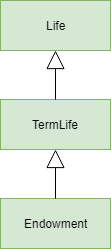
../_images/Inheritance1.png — Life, TermLife and Endowment#

The endowment policy pays out the maturity benefit of 1 at the end of its policy term. We have defined benefits cells as the expected value of benefits, so in addition to the death benefits considered in LifeTerm space, we’ll add the maturity benefit by overriding the benefits definition in Endowment space. In reality, the insured will not get both death and maturity benefits, but here we are considering an probabilistic model, so the benefits would be the sum of expected value of death and maturity benefits:

endowment = model.new_space(name='Endowment', bases=term_life)

@defcells
def benefits(x):
    if x < x0 + n:
        return d(x) / l(x0)
    elif x == x0 + n:
        return l(x) / l(x0)
    else:
        return 0

And the same operations on the Endowment space produces the following results:

>>> endowment.pv_benefits(50)
0
>>> endowment.frame
       pv_benefits  benefits              l      q           d
x
0     1.000000  0.003000  100000.000000    NaN  300.000000
0     0.997000  0.002991   99700.000000    NaN  299.100000
0     0.994009  0.002982   99400.900000    NaN  298.202700
0     0.991027  0.002973   99102.697300    NaN  297.308092
0     0.988054  0.002964   98805.389208    NaN  296.416168
0     0.985090  0.002955   98508.973040    NaN  295.526919
0     0.982134  0.002946   98213.446121    NaN  294.640338
0     0.979188  0.002938   97918.805783    NaN  293.756417
0     0.976250  0.002929   97625.049366    NaN  292.875148
0     0.973322  0.002920   97332.174218    NaN  291.996523
0     0.970402  0.970402   97040.177695    NaN         NaN
0     0.000000       NaN            NaN    NaN         NaN
NaN            NaN       NaN            NaN  0.003         NaN

You can see pv_benefits for all ages and benefits for age 60 show values different from TermLife as we overrode benefits.

pv_benefits(50) being 1 is not surprising. The disc_rate set to 1 in TermLife space is also inherited to the Endowment space. The discounting rate of benefits being 1 means by taking the present value of the benefits, we are simply taking the sum of all expected values of future benefits, which must equates to 1, because the insured gets 1 by 100% chance.

Dynamic spaces#

In many situations, you want to apply a set of calculations in a space, or a tree of spaces, to different data sets. You can achieve that by applying the space inheritance on dynamic spaces.

Dynamic spaces are parametrized spaces that are created on-the-fly when requested through call(()) or subscript([]) operation on their parent spaces.

To define dynamic spaces in a parent space, you create the space with a parameter function whose signature is used to define space parameters. The parameter function should return, if any, a mapping of parameter names to their arguments, to be pass on to the new_space method, when the dynamic spaces are created.

To see how this works, let’s continue with the previous example. In the last example, we manually set the issue age x0 of the policy to 50, and the policy term n to 10. We’ll extend this example and create policies as dynamic spaces with with different policy attributes. Assume we have 3 term life polices with the following attributes:

Policy ID	Issue Age	Policy Term
1	50	10
2	60	15
3	70	5

We’ll create this sample data as a nested list:

data = [[1, 50, 10], [2, 60, 15], [3, 70, 5]]

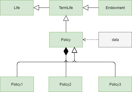
The diagram shows the design of the model we are going to create. The lines with a filled diamond shape on one end indicates that Policy model is the parent space of the 3 dynamic spaces, Policy1, Policy2, Policy3, each of which represents each of the 3 policies above. While Policy is the parent space of the 3 dynamic space, it is also the base space of them. Policy space inherits its members from Term model, and in turn Policy is inherited by the 3 dynamic spaces. This inheritance is represented by the unfilled arrowhead next the filled diamond.

Below is a script to extend the model as we designed above.

def params(policy_id):
    return {'name': 'Policy%s' % policy_id,
            'bases': _self}

policy = model.new_space(name='Policy', bases=term_life, formula=params)

policy.data = data

@defcells
def x0():
    return data[policy_id - 1][1]

@defcells
def n():
    return data[policy_id - 1][2]

The params function is passed to the constructor of the Policy space as the argument of formula parameter. The signature of params func is used to determine the parameter of the dynamic spaces, and the returned dictionary is passed to the new_space as arguments when the dynamic spaces are created. params is called when you create the dynamic subspaces of Policy, by calling the n-the element of Policy. params is evaluated in the Policy’s namespace. _self is a spacial reference that points to Policy.

The parameter policy_id becomes available within the namespace of each dynamic space.

In each of the dynamic spaces, the values of x0 and n are taken from data for each policy:

>>> policy(1).pv_benefits(50)
0.02959822305108317

>>> policy(2).pv_benefits(60)
0.04406717516109439

>>> policy(3).pv_benefits(70)
0.014910269595243001

>>> policy(3).frame
         n    x0           d  benefits              l  pv_benefits      q
x
NaN    5.0  70.0         NaN       NaN            NaN          NaN  0.003
 70.0  NaN   NaN  300.000000  0.003000  100000.000000     0.014910    NaN
 71.0  NaN   NaN  299.100000  0.002991   99700.000000     0.011910    NaN
 72.0  NaN   NaN  298.202700  0.002982   99400.900000     0.008919    NaN
 73.0  NaN   NaN  297.308092  0.002973   99102.697300     0.005937    NaN
 74.0  NaN   NaN  296.416168  0.002964   98805.389208     0.002964    NaN
 75.0  NaN   NaN         NaN  0.000000            NaN     0.000000    NaN
 76.0  NaN   NaN         NaN       NaN            NaN     0.000000    NaN

>>> policy.spaces
{'Policy1': <Space Policy[1] in Model1>,
 'Policy2': <Space Policy[2] in Model1>,
 'Policy3': <Space Policy[3] in Model1>}

Dynamic spaces of a base space are not passed on to the derived spaces. When a space is derived from a base space that has dynamically created subspaces, those dynamically created subspaces themselves are not passed on to the derived spaces. Instead, the parameter function of the base space is inherited, so subspaces of the derived space are created upon call(using ()) or subscript (using []) operators the derived space with arguments.

Reading Excel files#

You can read data stored in an Excel file into newly created cells. Space has two methods new_cells_from_excel and new_space_from_excel. new_space_from_excel is also available on Model. You need to have Openpyxl package available in your Python environment to use these methods.

new_cells_from_excel method reads values from a range in an Excel file, creates cells and populates them with the values in the range.

new_space_from_excel methods reads values from a range in an Excel file, creates a space, and in that space, creates dynamic spaces using one or some of the index rows and/or columns as space parameters, and creates cells in the dynamics spaces populating them with the values in the range.

Refer to the modelx reference for concrete description of those methods.

Exporting to Pandas objects#

If you have Pandas installed in your Python environment, you can export values of cells to Pandas’ DataFrame or Series objects. Spaces have frame property, which generates a DataFrame object whose columns are cells names, and whose indexes are cells parameters. Multiple cells in a space may have different sets of parameters. Generated