
Introduction to modelx#
modelx is a Python package to develop, run, debug and save complex numerical models using Python, just like you do with a spreadsheet. modelx is best suited for models in such fields as actuarial science, quantitative finance and risk management, where the calculation logic is expressed in recursive formulas.
modelx provides classes such as Model, UserSpace and Cells, for you to create their instances. Model, UserSpace and Cells are to modelx what Workbook, Worksheet and Range are to Excel.
A Cells object can be created from Python functions, and act like a cached function. A UserSpace object serves as a contanier of Cells objects, and provides the namespace for the contained Cells objects.
Here is a list of modelx’s main features:
A UserSpace can be quickly parameterized with names defined it, so that you can make multiple copies of the UserSpace dynamically
Quickly parameterize a UserSpace with names defined in it, and create dynamic copies of it
Quickly build object-oriented models, utilizing inheritance and composition
Trace formula dependency for debugging
Import and use any Python modules, such as Numpy, pandas, SciPy, scikit-learn, etc..
See formula traceback upon error and inspect local variables
Save models to text files and version-control with Git
Save data such as pandas DataFrames in Excel or CSV files within models
Auto-document saved models by Python documentation generators, such as Sphinx
Use Spyder with a plugin for modelx (spyder-modelx) to interface with modelx through GUI
To feel that modelx makes our life easier, let’s build a simple model using modelx.
A Quick Tour of modelx#
Building and running a model#
Let’s say we want to build a model that performs a Monte Carlo simulation to generate 10,000 stochastic paths of a stock price that follow a geometric Brownian motion and to price an European call option on the stock. For now, let’s ignore the fact that a Black-Scholes formula would give the analytical solution. Later, we will check the analytical method gives the same answer.
Here’s the entire script for building the model using modelx.
import modelx as mx
import numpy as np

model = mx.new_model()                  # Create a new Model named "Model1"
space = model.new_space("MonteCarlo")   # Create a UserSpace named "MonteCarlo"

# Define names in MonteCarlo
space.np = np
space.M = 10000     # Number of scenarios
space.T = 3         # Time to maturity in years
space.N = 36        # Number of time steps
space.S0 = 100      # S(0): Stock price at t=0
space.r = 0.05      # Risk Free Rate
space.sigma = 0.2   # Volatility
space.K = 110       # Option Strike


# Define Cells objects in MonteCarlo from function definitions
@mx.defcells
def std_norm_rand():
    gen = np.random.default_rng(1234)
    return gen.standard_normal(size=(N, M))


@mx.defcells
def stock(i):
    """Stock price at time t_i"""
    dt = T/N
    if i == 0:
        return np.full(shape=M, fill_value=S0)
    else:
        epsilon = std_norm_rand()[i-1]
        return stock(i-1) * np.exp((r - 0.5 * sigma**2) * dt + sigma * epsilon * dt**0.5)


@mx.defcells
def call_opt():
    """Call option price by Monte Carlo"""
    return np.average(np.maximum(stock(N) - K, 0)) * np.exp(-r*T)
After executing the code above from IPython console,
calling call_opt gives the price of the European option.
>>> call_opt()
16.26919556999345
call_opt is a Cells object, and it retains the returned value
until it needs to be recalculated.
It is not only call_opt that retains the returned value,
but also all the intermediate values used to calculate
the target call_opt are retained and available at no cost.
>>> stock(space.N)      # Stock price at i=N i.e. t=T
array([ 78.58406132,  59.01504804, 115.148291  , ..., 155.39335662,
        74.7907511 , 137.82730703])
If we want to see the option price for another strike, simply assign the new strike to K.
>>> space.K = 100   # Cache is cleared by this assignment

>>> call_opt()    # New option price for the updated strike
20.96156962064
You can dynamically create multiple copies of MonteCarlo
with different combinations of r and sigma,
by parameterizing MonteCarlo with r and sigma:
>>> space.parameters = ("r", "sigma")   # Parameterize MonteCarlo with r and sigma

>>> space[0.03, 0.15].call_opt()  # Dynamically create a copy of MonteCarlo with r=3% and sigma=15%
14.812014828333284

>>> space[0.06, 0.4].call_opt()   # Dynamically create another copy with r=6% and sigma=40%
33.90481014639403
Having the two copies of MonteCarlo make it easy to perform such tasks as comparing the values of the same items, such as the option price, or the stock price at any time before or at maturity, with different parameters. The dynamic UserSpaces are immutable, and destroyed when the base MonteCarlo is updated.
Closer look at the model#
Now, let’s look back and take a closer look at the initial script to understand more about what was going on when we built the model.
import modelx as mx
import numpy as np
The first import statement starts modelx behind the scene, and defines mx,
an alias for the modelx modules for convenience.
The second import statement should be familiar to most Python users.
It imports the numpy module as np into the global namespace of the __main__ module, which is the module that we are just working in.
As we will see later, defining np in the global namespace of __main__ doesn’t make it available from the Formulas.
By the next statement, we are creating a new Model object and assigning it
to a name model. Since we don’t give an explicit name to the new_model function,
the model is named Model1 by modelx.
A Model object is to modelx what a Workbook is to Excel.
It is the outermost container of all objects contained in it.
Then the next statement creates a UserSpace object named MonteCarlo in the model. A UserSpace is to modelx what a Worksheet is to Excel. It is a container in which we are going to create Cells objects.
model = mx.new_model()                  # Create a new Model named "Model1"
space = model.new_space("MonteCarlo")   # Create a UserSpace named "MonteCralo"
A Cells object acts like a cached function. It can be called like a function, and the returned value is retained until it needs to be updated. A Cells object resembles a cell in Excel, but unlike Excel’s cell, its formula can have parameters, so it can retain multiple values, one value for one set of parameter values.
A UserSpace has another important role, aside from being the parent of containing Cells, which is to provide the namespace for the Formulas of the containing Cells. In this sense, a UserSpace resembles a Python module.
A Cells object has an associated Formula object.
The Formula object is essentially a Python function,
except that it is not evaluated in the Python’s global namespace, which is, in our case,
__main__’s namespace, but instead,
it is evaluated in the namespace provided by the parent UserSpace.
You can define names in the UserSpace’s namespace by attribute assignment operations.
The next block of code assigns values and objects we use in our model to names in the namespace of MonteCarlo.
# Define names in MonteCarlo
space.np = np
space.M = 10000     # Number of scenarios
space.T = 3         # Time to maturity in years
space.N = 36        # Number of time steps
space.S0 = 100      # stock(0): Stock price at t=0
space.r = 0.05      # Risk Free Rate
space.sigma = 0.2   # Volatility
space.K = 110       # Option Strike
Internally, modelx keep these names and their values as Reference objects.
The next part constructs the main body of our model’s calculation logic.
It creates 3 Cells objects, std_norm_rand, stock and call_opt in MonteCarlo.
A Cells object acts like a cached function.
It can be called like a function, and the returned value is retained until
it needs to be updated.
defcells is a convenience decorator for creating Cells objects quickly
from function definitions.
The first def statement with defcells decorator creates a Cells
object named std_norm_rand, and assigns the object to the name std_norm_rand
in the global namespace of __main__.
In addition,
the statement defines the formula property of the Cells object from the std_norm_rand function definition. The formula property holds the Formula object,
which is essentially a copy of the decorated Python function,
but the global names in the Formula refer to the values we just assigned above.
The same goes with stock and call_opt.
Note that within the definitions of the formulas,
we can refer to the other Cells defined in MonteCarlo as well as the names defined above.
Also note that we can refer to the names directly,
without preceding object names and the dot.
# Create Cells objects in MonteCarlo and define their formulas from function definitions

@mx.defcells
def std_norm_rand():
    gen = np.random.default_rng(1234)
    return gen.standard_normal(size=(N, M))


@mx.defcells
def stock(i):
    """Stock price at time t_i"""
    dt = T/N
    if i == 0:
        return np.full(shape=M, fill_value=S0)
    else:
        epsilon = std_norm_rand()[i-1]
        return stock(i-1) * np.exp((r - 0.5 * sigma**2) * dt + sigma * epsilon * dt**0.5)


@mx.defcells
def call_opt():
    """Call option price by Monte Carlo"""
    return np.average(np.maximum(stock(N) - K, 0)) * np.exp(-r*T)
Debugging the model#
We often need to debug models we build to make sure their results are correct. modelx has features to help us with such debugging.
One of such features is modelx’s capability to trace calculation dependency.
The precedents method on Cells returns a list of precedents
for given arguments. The list contains
References and Nodes, which represents Cells associated with arguments,
that are used by the arguments and the Cells.
Continuing from the above example, below shows the precedents
of call_opt() and stock(36).
>>> call_opt()    # Make suer this is run.
20.96156962064

>>> call_opt.precedents()   # Returns precedents of call_opt()
[Model1.MonteCarlo.stock(i=36)=
 array([ 78.58406132,  59.01504804, 115.148291  , ..., 155.39335662,
         74.7907511 , 137.82730703]),
 Model1.MonteCarlo.np=<module 'numpy' from 'C:\\Users\\...\\__init__.py'>,
 Model1.MonteCarlo.N=36,
 Model1.MonteCarlo.K=100,
 Model1.MonteCarlo.r=0.05,
 Model1.MonteCarlo.T=3]

>>> stock.precedents(36)     # Reteruns precedents of stock(36)
[Model1.MonteCarlo.std_norm_rand()=
 array([[-1.60383681,  0.06409991,  0.7408913 , ...,  0.82163882,
         -0.49991377,  1.17804635],
        [-0.67804259,  1.35072849,  2.07565699, ...,  0.32146055,
         -0.7599273 ,  1.73113515],
        [-1.42381038, -0.36400253, -0.55303109, ...,  0.04814081,
         -1.19998129, -0.08490359],
        ...,
        [-2.12588633, -0.19431652, -1.68358751, ..., -0.3466555 ,
         -0.10290633, -0.68737272],
        [-1.32955138,  0.28343894, -2.01866314, ...,  1.58520134,
          0.30001717, -0.63270348],
        [ 2.02929671, -1.42904385,  0.26366402, ..., -0.05042656,
          0.14542656, -0.21076562]]),
 Model1.MonteCarlo.stock(i=35)=
 array([ 69.72140666,  63.93061459, 113.12553545, ..., 155.45729533,
         73.98023943, 139.16636139]),
 Model1.MonteCarlo.T=3,
 Model1.MonteCarlo.N=36,
 Model1.MonteCarlo.np=<module 'numpy' from 'C:\\Users\\...\\__init__.py'>,
 Model1.MonteCarlo.M=10000,
 Model1.MonteCarlo.S0=100,
 Model1.MonteCarlo.r=0.05,
 Model1.MonteCarlo.sigma=0.2]
Conversely, succs method returns a list of Nodes that are
using, for example, sock(36):
>>> stock.succs(36)
[Model1.MonteCarlo.call_opt()=20.96156962064]
Another feature of modelx makes it easy to trace errors.
When an error is raised in a Cells call,
modelx prints out the traceback of the call.
Let’s intentionally make stock(10) raise an error just before returning
by inserting a raise statement.
@mx.defcells
def stock(i):
    """Stock price at time t_i"""
    dt = T/N
    if i == 0:
        return np.full(shape=M, fill_value=S0)
    else:
        epsilon = std_norm_rand()[i-1]
        if i == 10:
          raise ValueError('Error raised')
        return stock(i-1) * np.exp((r - 0.5 * sigma**2) * dt + sigma * epsilon * dt**0.5)
Execution of call_opt eventually reaches stock(10) when the error is raised.
The error message prints out the traceback of the execution.
>>> call_opt()
...
FormulaError: Error raised during formula execution
ValueError: Error raised

Formula traceback:
0: Model1.MonteCarlo.call_opt(), line 3
...
25: Model1.MonteCarlo.stock(i=12), line 10
26: Model1.MonteCarlo.stock(i=11), line 10
27: Model1.MonteCarlo.stock(i=10), line 9

Formula source:
def stock(i):
    """Stock price at time t_i"""
    dt = T/N
    if i == 0:
        return np.full(shape=M, fill_value=S0)
    else:
        epsilon = std_norm_rand()[i-1]
        if i == 10:
          raise ValueError('Error raised')
        return stock(i-1) * np.exp((r - 0.5 * sigma**2) * dt + sigma * epsilon * dt**0.5)
In addition, the trace_locals function
helps to inspect the values of the local variables held when the error is raised.
>>> mx.trace_locals()
{'i': 10,
 'dt': 0.08333333333333333,
 'epsilon': array([-0.52430375, -1.29168268,  0.04276587, ..., -0.45993114,
         1.33283969,  0.26335339])}
Saving the model#
A Model can be saved as files in a directory tree or as just one zip file,
by write or zip method.
>>> model.write(r'C:\Users\mxuser\Model1')

>>> model.zip(r'C:\Users\mxuser\Model1.zip')
The contents of the directory tree are written as a pseudo Python package, and
the UserSpaces are output in __init__.py in sub directories
as if they are Python modules,
and the Cells are output as if they are Python functions.
This means that we can version-control the output of the model using Git
as if they are Python code, and auto-document it from the
docstrings using a document generator, such as Shpinx.
Using modelx with Spyder#
Spyder is a popular open-source Python IDE, and it allows plugins to be installed to add extra features to itself. The Spyder plugin for modelx, which is avaialble as a separate pacakge, enriches user interface to modelx in Spyder. The plugin adds custom IPython consoles and GUI widgets for using modelx in Spyder.
Using Spyder and the plugin, the sample model is shown as a tree in a GUI widget:
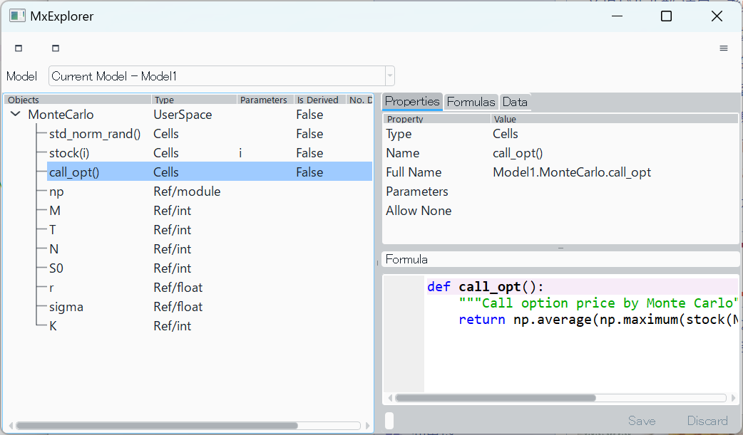
Sample model in Spyder#
The widget makes it easy to edit the model. Other widgets installed by the plugin help to view data of modelx objects and analyze the dependency of them. For more on the plugin, see Spyder plugin.
Overview of modelx objects#
As we have seen in the quick tour above, modelx lets us build models composed of a few types of objects. Model, UserSpace, Cells, Reference are the most frequent types we use. In this section we briefly review these types of objects to have basic understanding of them.
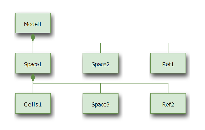
The diagram below illustrates containment relationships between those objects.
Models, Spaces and Cells#
Models are the top level container objects. Models can be saved to files and loaded back again. Multiple models can be opened in one Python session at the same time.
Within a model, we can create UserSpace objects.
UserSpace objects are editable.
There are read-only types of space objects, such as ItemSpace and DynamicSpace.
For example, in the quick tour above, we have created
two ItemSpace objects, MonteCarlo[0.03, 0.15] and MonteCarlo[0.06, 0.4]:
>>> space[0.03, 0.15].call_opt()  # space refers to the MonteCarlo space
14.812014828333284

>>> space[0.06, 0.4].call_opt()
33.90481014639403
Collectively, we call them Space objects, or just spaces, whether they are of the editable or read-only types.
Spaces serve as containers, separating contents in the model into components. the spaces can contain Cells, Reference objects and other Space objects, allowing a tree structure to form within the model. The spaces also serve as the namespaces for the formulas associated to the spaces themselves or to the Cells objects contained in them.
We call Cells objects just cells. A cells is an object that has one formula and can hold its value, just like spreadsheet cells can have formulas and values. But unlike spreadsheet cells, in modelx, a cells value is either calculated by its formula or assigned as an input by the user for each argument. When an input value is assigned by the user, its fomula is not calculated for the argument.
Reference objects are names bound to arbitrary objects.
We call Reference objects, references, or just refs.
References can be defined either in spaces or in models.
References defined in a space can be referenced from
the formulas of the cells defined in the space,
or the formula associated with the space.
For example, Cells1.formula (and Space1.formula if any) can
refer to Ref2.
References defined in a model (for example Ref1 in the
diagram above) can be referenced from formulas
defined anywhere in the model, unless other references
override the name binding defined by the reference in the model.